Balsn CTF 2021: dlog

@blackb6a played Balsn CTF 2021 last weekend. There are three crypto challenges, and they are all pretty hard. In this blog post we will cover the dlog challenge, which is a timing attack on the CPython's pow method. @grhkm2023 and I spent a lot of time working on this challenge. Although we did not solve it, we actually learned a lot from the challenge and lost a pile of hair (maybe it is just me).

By the way, I am still solving the challenge (and making the attack stable) while compiling the writeup and meanwhile there were many questions arose. Would it be fun or troublesome reading through? I genuinely don't know.

Challenge Summary⌗

Suppose that $p = 2q+1$ where $p, q$ are primes. Let also $s$ be an exponent. We are given that $0 < p < 2^{1025}$ and $0 < s < 2^{100}$. Given three APIs:

• /oracle receives $x$ and returns $x^s\ \text{mod}\ p$,
• /flag receives $x$. If $x^s\ \text{mod}\ p = 1337$ the flag will be returned,
• /metrics returns metrics including the total number of calls and the total time on processing /oracle and /flag.

The objective is to retrieve the flag.

Solution⌗

Part I: Recovering modulus $p$⌗

It is easy to recover $p$. We can simply send $x = -1$ to /oracle. If $s$ is odd, then

\[x^s\ \text{mod}\ p = (-1)^s\ \text{mod}\ p = p - 1.\]

The prime $p$ they used is a safe prime, i.e., $p = 2q+1$ for another prime $q$. That said, the order of the subgroups could either be $1$, $2$, $q$ or $2q$.

Part II: Timing attacking in disguise⌗

The /metrics API immediately suggested us that this challenge is a timing attack because we can see oracle_processing_seconds_sum being the total time processing all the /oracle calls. To be exact, we can compute the time to compute pow(1337, s, p) with the following steps:

1. Call /metrics and get the values of oracle_processing_seconds_count (denoted as $n_1$) and oracle_processing_seconds_sum (denoted as $t_1$).
2. Call /oracle?x=1337.
3. Call /metrics and get the values of oracle_processing_seconds_count (denoted as $n_2$) and oracle_processing_seconds_sum (denoted as $t_2$).
   • If $n_2 = n_1 + 1$ (i.e., there are no oracle calls triggered by others), then the time to compute pow(1337, s, p) is $t_2 - t_1$.
   • Otherwise set $n_1 \leftarrow n_2$ and $t_1 \leftarrow t_2$ and go back to step 2.

As an example, the sampled times to compute pow(1, s, p), pow(1337, s, p) and pow(2**1024, s, p) are respectively 0.12ms, 0.50ms and 0.77ms.

Part III: Understanding CPython's pow function⌗

To explain the difference in the computing time, we need to read code for pow for CPython 3.9. If the exponent s does not exceed 240 bits, it would use the below algorithm to compute pow(x, s, p)¹. This is the case for this challenge:

1. Denote $z \leftarrow 1$ and let $k \in \mathbb{N}$ such that $2^{30(k-1)} \leq s < 2^{30k}$.
2. For each $b = 30k-1, 30k-2, ..., 1, 0$,
   • Compute $z \leftarrow z \cdot z\ \text{mod}\ p$.
   • If $s \land b \neq 0$, then compute $z \leftarrow z \cdot a\ \text{mod}\ p$.
3. Return $z$.

Python uses Karatsuba algorithm for multiplication. If we are multiplying two $n$-bit numbers, the time complexity would be $\mathcal{O}(n^{\log_23}) \approx \mathcal{O}(n^{1.585})$. On the other hand, the time complexity to compute $a\ \text{mod}\ p$ (where $a$ and $p$ are $n$-bit long) is $\mathcal{O}(n^2)$, unless $\left|a\right| < \left|p\right|$ - which would be $\mathcal{O}(n)$ (for copying the digits).

Part IV: Taking the first step to recover s⌗

Let $\overline{s_1 s_2 ... s_b}$ be the binary representation of $s$ ($s_1 = 1$). With the algorithm stated above, we have the below graph those record the intermediate values of $z$:

Since the time to take a reduction (i.e., perform modulo $p$) is $\mathcal{O}(n^2)$ whenever the number is larger than $p$, we expected that we could detect whether a reduction is taken place.

For example, if we have $a_1$ such that ${a_1}^2\ \text{mod}\ p$ is small enough, then $z \leftarrow z \cdot z\ \text{mod}\ p$ would take the fast path when $z \leftarrow z \cdot z\ \text{mod}\ p$. In the below graph, the path with ✨ will be taken when $s_2 = 0$. Since it takes one less reduction, it is faster. On the other hand, the fast path is not triggered when $s_2 = 0$.

We could detect whether $s_2 = 0$ by checking if the fast path is taken. We thought it is hard to determine if a single fast path is triggered, since it could only affect less than 1% of the total time. We tried it nonetheless as we were out of ideas. On the other hand, we also look for $a_2$ such that $z = {a_2}^2\ \text{mod}\ p$ is small. In that way, another path (labeled with ✨) will be triggered - and it is a fast path.

Define $\mathcal{T}(x)$ be the time to compute pow(x, s, p). Now let's draft the algorithm $\mathcal{A}$ to determine if $s_2 = 0$ or $s_2 = 1$:

1. Denote $c_1 \leftarrow 0$ and $c_2 \leftarrow 0$.
2. Repeat 500 times:
   • Generate random $a_1, a_2 \in \mathbb{Z}_p$ such that ${a_1}^2\ \text{mod}\ p$ and ${a_2}^3\ \text{mod}\ p$ are small.
   • Let $t_1 = \mathcal{T}(a_1)$ and $t_2 = \mathcal{T}(a_2)$.
   • If $t_1 < t_2$ then assign $c_1 \leftarrow c_1 + 1$, otherwise assign $c_2 \leftarrow c_2 + 1$.
3. If $c_1 \gg c_2$, then we know that $s_2 = 0$. If $c_1 \ll c_2$, then $s_2 = 1$. Otherwise we cannot tell (statistically) what $s_2$ is.

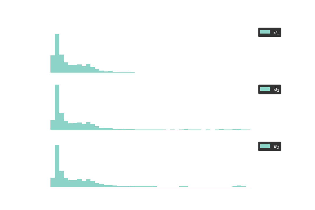
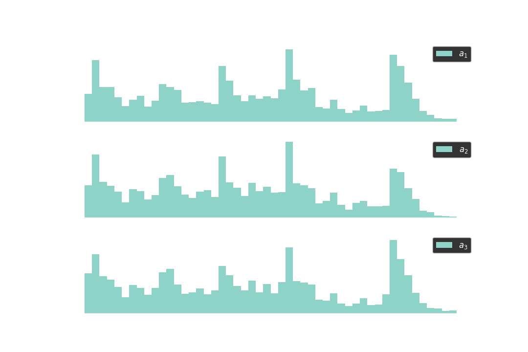
After all, the below histograms show the distribution for the sampled computation times of 10K different sets of $a_1, a_2, a_3 \in \mathbb{Z}_p$, where

• ${a_1}^2\ \text{mod}\ p < 2^{512}$,
• ${a_2}^3\ \text{mod}\ p < 2^{512}$, and
• $a_3$ is not constrainted (as the control group).

As seen from the histograms, it is faster to compute pow(a1, s, p) than to compute pow(a2, s, p). That said, the second most significant bit, $s_2$, would be a zero.

Part V: Completing the attack⌗

Now we have $s_2 = 0$. To proceed further, we can find $a_1, a_2 \in \mathbb{Z}_p$ such that ${a_1}^4\ \text{mod}\ p$ and ${a_2}^5\ \text{mod}\ p$ are both small. The red path will be taken if $s_3 = 0$ and otherwise the blue path. We can use the times to compute pow(a1, s, p) and pow(a2, s, p) to identify whether the red or the blue path is triggered.

In general, suppose that the prefix of $s$ being $s_\text{prefix} = \overline{s_1s_2...s_k}$, we can identify $s_{k+1}$ by finding $a_1, a_2 \in \mathbb{Z}_p$ such that

\[{a_1}^{2s_\text{prefix}}\ \text{mod}\ p\quad\text{and}\quad{a_2}^{2s_\text{prefix} + 1}\ \text{mod}\ p\]

are both small. To minimize the remote calls, I tried to find the remaining bits via the baby-step giant-step algorithm after I recovered 60 bits of $s$. Anyway this is my script for recovering 60 bits:

challenge = Challenge()

p = challenge.oracle(-1)[0] + 1
q = (p-1) // 2

s_prefix = 1

while s_prefix.bit_length() < 60:
    e1 = 2 * s_prefix
    e2 = 2 * s_prefix + 1

    d1 = pow(e1, -1, q)
    d2 = pow(e2, -1, q)

    while True:
        b1 = random.getrandbits(512)
        a1 = pow(b1, d1, p)

        if pow(a1, e1, p) == b1: break

    while True:
        b2 = random.getrandbits(512)
        a2 = pow(b2, d2, p)

        if pow(a2, e2, p) == b2: break

    t1 = challenge.oracle(a1)[1]
    t2 = challenge.oracle(a2)[1]

    s_prefix *= 2
    if t1 > t2: s_prefix += 1

    assert bin(s).startswith(bin(s_prefix))

Final words⌗

The attack largely depends on the fluctuation of the measured times, which made the attack very unstable. There's something to do with statistics on this part, but I do not have a workaround just yet. Anyway, there are chances to win the flag with the idea, but unfortunately the variance lowers the probability a lot.

We found some papers like "A practical implementation of the timing attack" by J.-F. Dhem, F. Koeune, P.-A. Leroux, P. Mestré, J.-J. Quisquater and J.-L. Willems. Maybe I should take it a look later, too.